Dan Turkel
Perceptibility of Lossy Audio Encoding as a Signal Detection Problem
Nota bene: The below was written as a response paper relating material from a course on perception to my own interests. I may have gone a bit overboard. The experimental component is not meant to be a verdict on claims of transparency for audio compression methods. Instead, I hope to demonstrate how signal detection theory provides a useful toolkit for studying lossy compression.
Introduction
As a music-lover and a technophile, I am fascinated the way we digitize and then recreate analog sound signals. Today, unless we listen to a tape player or vinyl record, we get just about all of our music in digital form, which means that the sound must make the transformation from analog pressure wave to a digital representation of that wave that we store, and then back to an analog wave that comes out of our speakers. While technological advances have given us a great ability to losslessly encode analog waves such that they can be perfectly reconstructed without any change in the signal, most of the time we listen to lossy encodings, which toss out certain pieces of the signal deemed to be psychoacoustically irrelevant. I decided to investigate lossy audio encoding as a signal detection problem: can the errors introduced in lossy compression (sound artifacts, missing frequencies) be reliably detected under experimental conditions?
This experiment is partially motivated by the increased visibility of a variety of digital encodings for music files, which has spurred a greater desire to understand these formats. Widespread high-bandwidth internet means that music retailers are offering music downloads in more than just the smallest formats. When a voracious consumer of music like myself goes to the popular website BandCamp to purchase music, he is greeted with two “standard high-quality formats” (MP3 VBR V0 and MP3 CBR at 320 kbps) and four for “audiophiles and nerds” (FLAC, AAC, Ogg Vorbis, and ALAC). Examining the discernibility of lossy audio encoding allows us to better establish the meaning and importance (or lack thereof) of these choices.
Overview of Digital Audio
An analog sound wave is a time-varied continuous function of air pressure in the transmitting medium—generally air. To store that wave digitally, we make two compromises because we only have finite digital storage space. We have to pick a frequency at which we will “sample” the original wave (assign the signal at that time a numeric value) because we cannot have an infinite number of signal values per second, and we must choose a finite range of discrete values which each sample can fall into because if each value is allowed to be infinitely high or low, then each sample would require infinite space to store that value (because the digital “word-length” of each sample’s value has to be pre-determined in order to know when the next sample’s value begins). The standard for audio on CDs is a 44.1 kHz sampling rate and two channels of 16-bit resolution values. These values are sufficiently high that, by the Nyquist-Shannon Sampling Theorem, we can perfectly recreate analog signals with constituent frequencies in the range of human hearing (about 20 Hz – 20 kHz) from their digital representatives (Shannon, 1998).1 Furthermore, lossless digital signals can even be compressed by complex algorithms to take up substantially less digital space without losing any of the uncompressed signal in a process called lossless compression.
However, most popular digital audio formats like MP3 deliberately toss out information from the original signal that is thought to be psychoacoustically imperceptible in order to save on storage space. Thus, sounds that are either outside the range of human hearing, or sounds that should not be perceptible in the presence of the rest of the signal are removed from the signal or stored with less precision (see Figure 2).2 This is called a “lossy” encoding method because information from the original signal is lost and errors can be introduced as precision is lowered. Lossy compression is designed to be minimally perceptible, but since lossy encoding schemes are available in a wide variety of compression levels, the perceptibility should be expected to vary. I decided to experiment on myself using MP3 files encoded from a lossless digital file at 128 kilobits per second (kbps), which is about 1/11th of uncompressed 16 bit audio × 44.1 kHz × 2 channels = 1411.2 kbps (though the lossless source file was encoded with lossless compression, so its actual bitrate would be less than the theoretical 1411.2 kbps and the original-to-MP3 ratio would be less than 11). This bitrate was chosen as 128 kbps is on the low end of the range of common MP3 encodings.
Experiment
I took lossless digital copies of three songs and trimmed them to roughly 30-second sections in Audacity (Audacity Team, 2014) and saved the shortened version in a lossless format so that there was no signal loss in the trimming process. Next I created a lossy MP3 copy of the trimmed version using XLD (tmkk, 2014) at constant 128 kbps bitrate. Lastly, I took my lossless trimmed version and converted it to a second lossless format (from FLAC to WAV) so that it would be compatible with the double-blind testing software; this step also featured no signal loss from the original. I then loaded the lossless and lossy trimmed files into Lacinato ABX (Connor, 2014). I listened several times to both versions (using Audio Technica M50 headphones at 44% volume) of the clip to acclimate myself to their differences to the best of my ability and then ran the “ABX Test” in ABX where it presented me with an unlabeled clip X and I had to determine whether it was clip A (lossless) or B (lossy). I did 20 trials of this and then viewed my results. (See Figure 4 for a summary illustration of the experimental process.)
Results
The first clip I tested was from the song “Before I Leave” by Christian Fennesz. The song is electronic and features sections of fairly rapid pulses of identical simple sounds. Due to the precise nature of the song’s sound, I suspected that it would likely be easy to pick out any imprecisely timed noise that was added in the lossy encoding process. As I listened to each version several times to acclimate myself, I immediately picked up on some noticeable noise present in the MP3. Indeed, in testing, I was able to correctly determine all 15 lossless X clips and 5 lossy X clips (the software does not allow you to ensure that the output is 50% A and 50% B). I deemed compression noise and quality decrease to be the “signal” to be detected, so I had a hit rate (signal properly detected) of 100% and a correct rejection rate (signal not detected when not present) of 100%, with no misses or false positives. Additionally, since I did 20 trials and was correct on all of them, the ABX software calculated a confidence of .99999905 that my performance was better than chance, which indicates near-certainty that the lossy compression was detectable. See Figures 1 – 3 for illustration of the spectral difference between the lossless and lossy clips of “Before I Leave.”
The next clip was from the song “Phantom Other” by Department of Eagles. Compared to “Before I Leave,” “Phantom Other” is incredibly complex, featuring guitar, bass guitar, acoustic drums, synthesizers, and several layers of vocals. Orienting myself to the lossless and lossy versions of the clip, I decided that the only real difference I could notice was that the bass drum and bass guitar blended together a bit more in the lossy version than in the lossless. After 20 trials, of which 9 were actually lossless and 11 of which were actually lossy, I had an accuracy rating of 65% (13/20), which is not much greater than the expected 50% for random guessing. Indeed, the calculated confidence was only .868412018 that my performance was better than chance, which is not nearly enough to claim that the difference is detectable. My hit-rate was 72%, so I correctly identified the lossy clip 8 times out of 11 (and missed 3 times), but my correct rejection rate was 55%, meaning that I only correctly stated that the lossless clip was lossless 5 out of 9 times (and gave false positives the other 4).
The last clip was from the song “My Valuable Hunting Knife” by Guided by Voices. Unlike the precision of “Before I Leave” or the complex production of “Phantom Other,” “My Valuable Hunting Knife” was recorded on cheap four- and eight-track tape machines.3 I had suspected that since the original clip already had errors resultant from the inherently lossy (or “lo-fi”) recording process (like an odd bit of vocal distortion 6 seconds into my clip) that it would be hard to pick out new errors introduced in the conversion process. However, when acclimating myself to the two clips, I was able to detect some hissing and compression artifacts under the vocals in the lossy version of the clip and I was once again 100% accurate in detecting the 16 lossless and 4 lossy clips (though it is unfortunate that the distribution should have been so uneven) with the same confidence level as “Before I Leave.” It is possible that starting with a lo-fi clip results in more exaggerated errors once lossy compression is added.
Discussion
From my fairly simple experiment, it seems that the ability to detect introduced errors and loss of information from lossy audio encoding is highly contingent on (at least) the clip itself. A track with high precision and regularity (“Before I Leave”) make it easy to pick out out-of-place errors and a track with lo-fi production (“My Valuable Hunting Knife”) seemed to lead to exaggerated compression artifacts after lossy encoding. On the other hand, a track with high production value and a large quantity of instruments (“Phantom Other”) did not feature any discernible errors or signal loss suitably reliable for determining whether or not a clip was lossy.
On top of these factors, it seems likely that choice of listening equipment, volume, encoding method and quality setting, and even choice of subject (listener) would lead to potentially dramatic variety in ability to discern lossy audio encoding.4 Indeed, the importance of lossless versus lossy audio files for listening purposes (as opposed to archival purposes) has been frequently debated, with lossless detractors claiming that the larger file size is not worth the often unnoticeable difference. Meyer and Moran studied the ability to discern the difference between high resolution (both bitrate and sample rate) Super Audio CDs (SACDs) and the same SACDs modified to have standard CD quality resolution and found that the accuracy rating in their ABX test was 49.82% (276 correct out of 554 trials), indicating results effectively the same as chance (Meyer, 2007, p. 777). Furthermore, filtering the results by various demographic elements produced no hidden correlations.
The discussion of discernibility of audio reproduction quality is also often used to critique expensive audio equipment. A user of the Audioholics forum for audiophiles claimed in a now-(in)famous post to have been part of an informal study where several self-proclaimed audiophile listeners not only could not reliably discern the difference between audio played through a mid-priced speaker cable by cable brand Monster and standard stranded-copper speaker wire, but could not even discern the difference when the ordinary speaker wire was replaced (without their knowledge) with straightened metal coat hangers (Dean, 2004). Naturally, studies like this draw criticism from those who feel that high-price audio equipment creates a noticeable difference in playback quality and the debate will likely continue with anecdotal and scientific evidence from both sides for the foreseeable future.
Conclusion
Signal detection theory provides a framework for the study of perceptive systems and has a vast array of applications from telecommunications to email spam-detection to interface design. The experiment in this paper presents just a small example of how audio reproduction is a site ripe for rich analysis with signal detection theory, even if it does not conclusively tell the reader which format to pick for their next album download.
Files
You can download the files I used for the ABX test in a zip file right here. As mentioned in the text, I used Lacinato ABX (available for all OS X/Windows/Linux) for my testing, though there are many alternatives available online. Feel free to share your results with me at if you decide to test yourself!
Figures
All spectrograms produced using Spek (Kojevnikov, 2014).
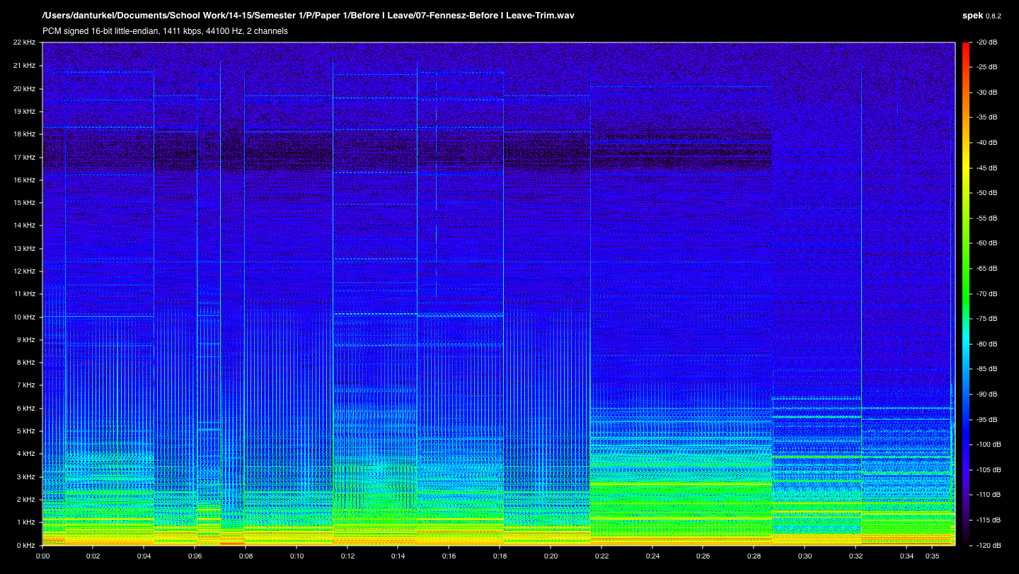
Figure 1: The spectrogram of the lossless clip of “Before I Leave.” The x-axis represents time, the y-axis represents frequency, and the color represents amplitude. The song’s precise repetitive nature can be seen in the evenly spaced vertical lines, with tone and sound changes indicated by abrupt shape changes. (Click image for full size.)
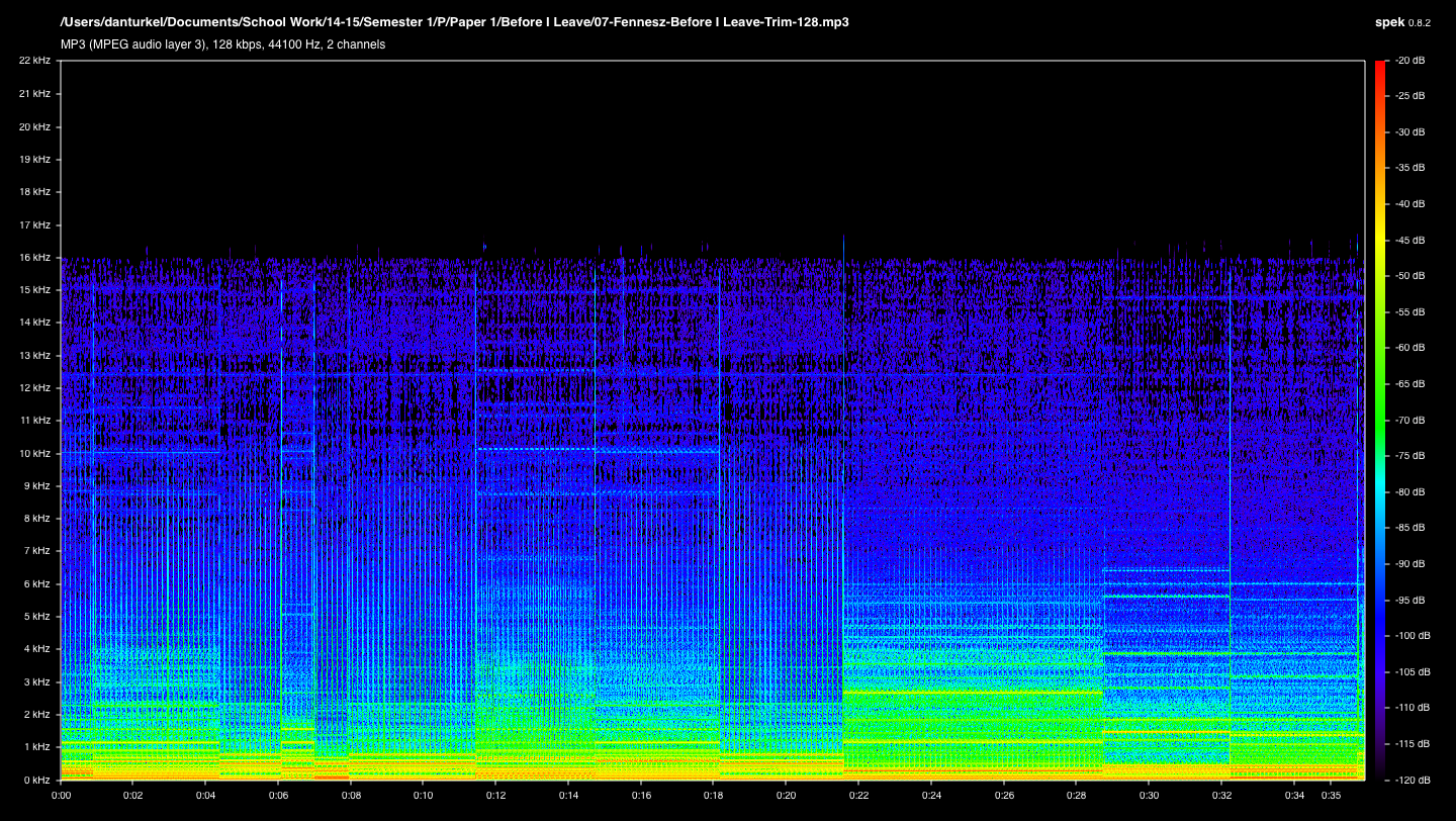
Figure 2: The spectrogram of the lossy clip of “Before I Leave.” Notice that all frequencies above 16kHz have been completely removed. Additionally, bands of frequency have been attenuated on the higher-end of the remaining spectrum. (Click image for full size.)
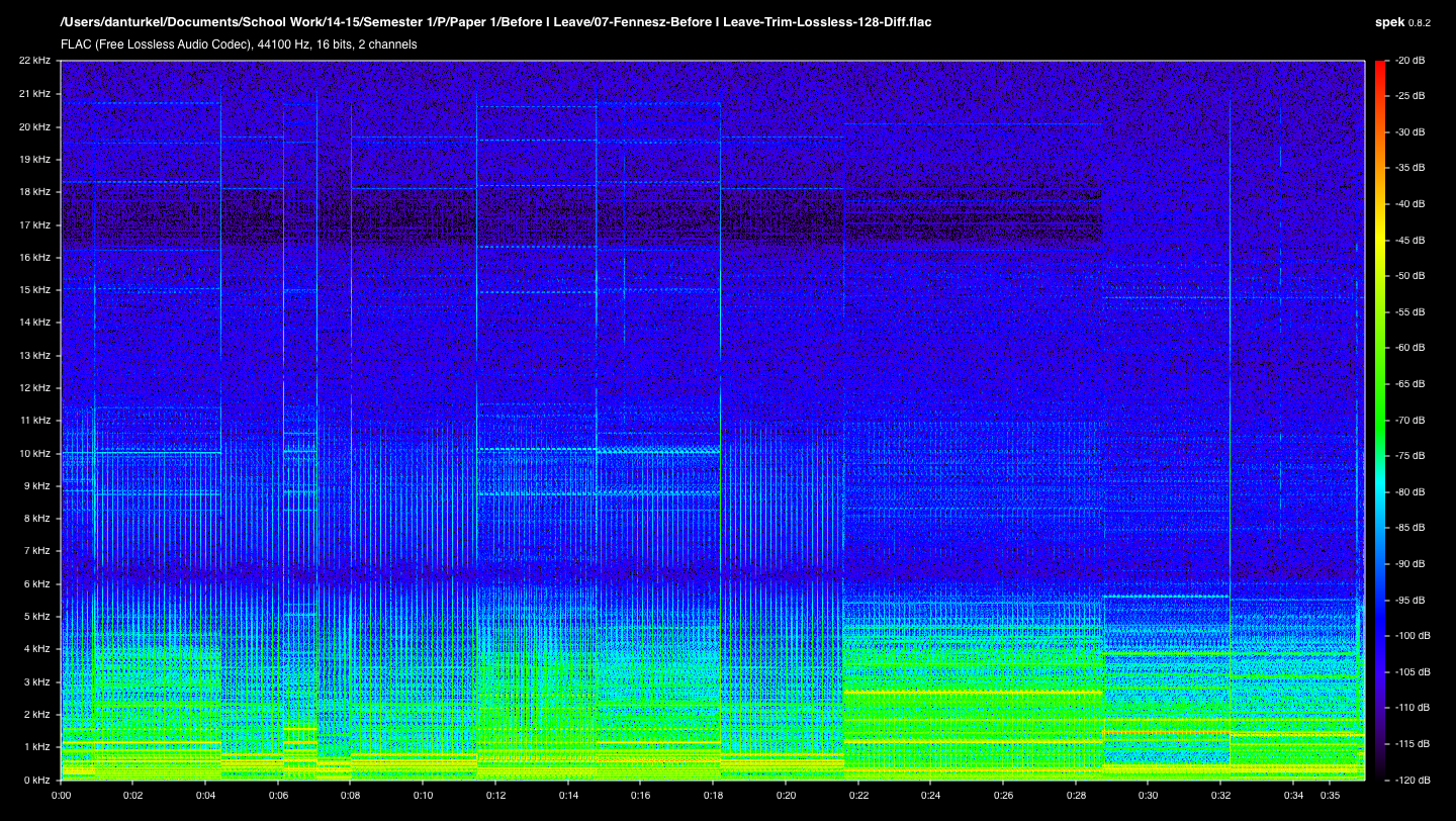
Figure 3: The spectrogram of the difference between the lossless and the lossless clips of “Before I Leave.” The image was created by inverting the signal (i.e. multiplying the entire signal by -1) of the lossy copy and adding it to the lossless copy so that only the differences between the two remain. Since lossy encoding dramatically changes the precision of the waveform and attenuates to varying degrees signals all across the spectrum, this spectrogram can be misleading and make the difference appear much larger than it is. However, the horizontal white bars around 9 and 10 kHz in the first half of the clip show us an area of moderate signal difference that stands out from the background difference noise. (Click image for full size.)
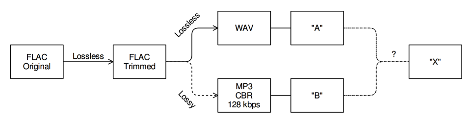
Figure 4: The procedure by which the two clips were prepared and tested.
Footnotes
-
The theorem specifically states that if a function with no frequencies higher than x Hz can be completely recreated from a digital representation with sampling rate 2x Hz (or higher). The sampling rate in CD audio is 44.1 kHz, so CDs can theoretically completely recreate signals with constituent frequencies 22.5 kHz or lower, which covers the entire range of human hearing. In reality, imperfections at any point in the signal chain interfere with perfect recreation. ↩
-
An in-depth explanation of how the MP3 encoder determines what can be tossed out or represented with less detail is out of the scope in this paper. However, Wilburn (2007) provides a good overview of the compression: the signal is broken down into several frequency bands which are analyzed for psychoacoustic perceptibility and compressed with precision proportional to the perceptibility of that frequency band in a given period of time. The result is that frequency bands which are very perceptible in a given period are stored with high precision, but frequency bands which are not very perceptible in a given period are stored with low precision, which saves space. ↩
-
“The advance for [“My Valuable Hunting Knife” album] Alien Lanes was close to a hundred thousand dollars. The cost for recording Alien Lanes, if you leave out the beer, was less than ten dollars,” (Greer, 2005, p. 96). ↩
-
This hypothesis is suggested by Benjamin as well, regarding an examination into just-noticeable-difference bitrate thresholds: “Conducting a reliable experiment regarding the bit rate threshold at which the music becomes distinguishably different is outside the scope of this analysis. The pursuit in itself seems somewhat futile as the answer will always depend on subjective factors such as the quality of the listener’s sound system and how attuned his or her ear is to the music” (2010, p. 16). ↩
References
Audacity Team, The. (2014). Audacity (Version 2.0.6) [Software]. Available from <Sourceforge>.
Benjamin, A. (2010, December 9). Music Compression Algorithms and Why You Should Care. Department of Electrical and Systems Engineering. Retrieved October 3, 2014, from <WUSTL (PDF)>.
Connor, C. (2014). Lacinato ABX/Shootout-er (Version 2.33) [Software]. Available from <Lacinato>.
Dean, B. (2004, June 24). Speakers; When is good enough, enough. Audioholics Home Theater Forums. Retrieved October 5, 2014 from <Audioholics>.
Greer, J. (2005). Guided By Voices: Twenty-one Years of Hunting Accidents in the Forests of Rock and Roll [Google Books version]. Retrieved from <Google Books>.
Kojevnikov, A. (2014). Spek: Acoustic Spectrum Analyzer (Version 0.8.2) [Software]. Available from <Spek>.
Meyer, E. B., & Moran, D. R. (2007). Audibility of a CD-Standard A/D/A Loop Inserted into High-Resolution Audio Playback. Journal of the AES, 55(9), 775-779. Retrieved October 3, 2014, from <Drew Daniels (PDF)>.
Montgomery, C. (2012, March 1). 24/192 Music Downloads...and why they make no sense. Xiph.org. Retrieved October 3, 2014, from <xiph.org>.
Shannon, C. E. (1998). Communication In The Presence Of Noise. Proceedings of the IEEE, 86(2), 447-457. Retrieved October 4, 2014, from <Stanford (PDF)>.
Reprint of the original 1949 paper.
tmkk. (2014). XLD: X Lossless Decoder (Version 147.0) [Software]. Available from <tmkk>.
The author of the software is known only as “tmkk.” The MP3 encoding performed for the peformed in XLD was done using the built-in LAME encoder, which features code from The LAME Development Team.
Wilburn, T. (2007, October 4). The AudioFile: Understanding MP3 compression. Ars Technica. Retrieved October 4, 2014, from <Ars Technica>.